Bullet simulation

Bullet is on field

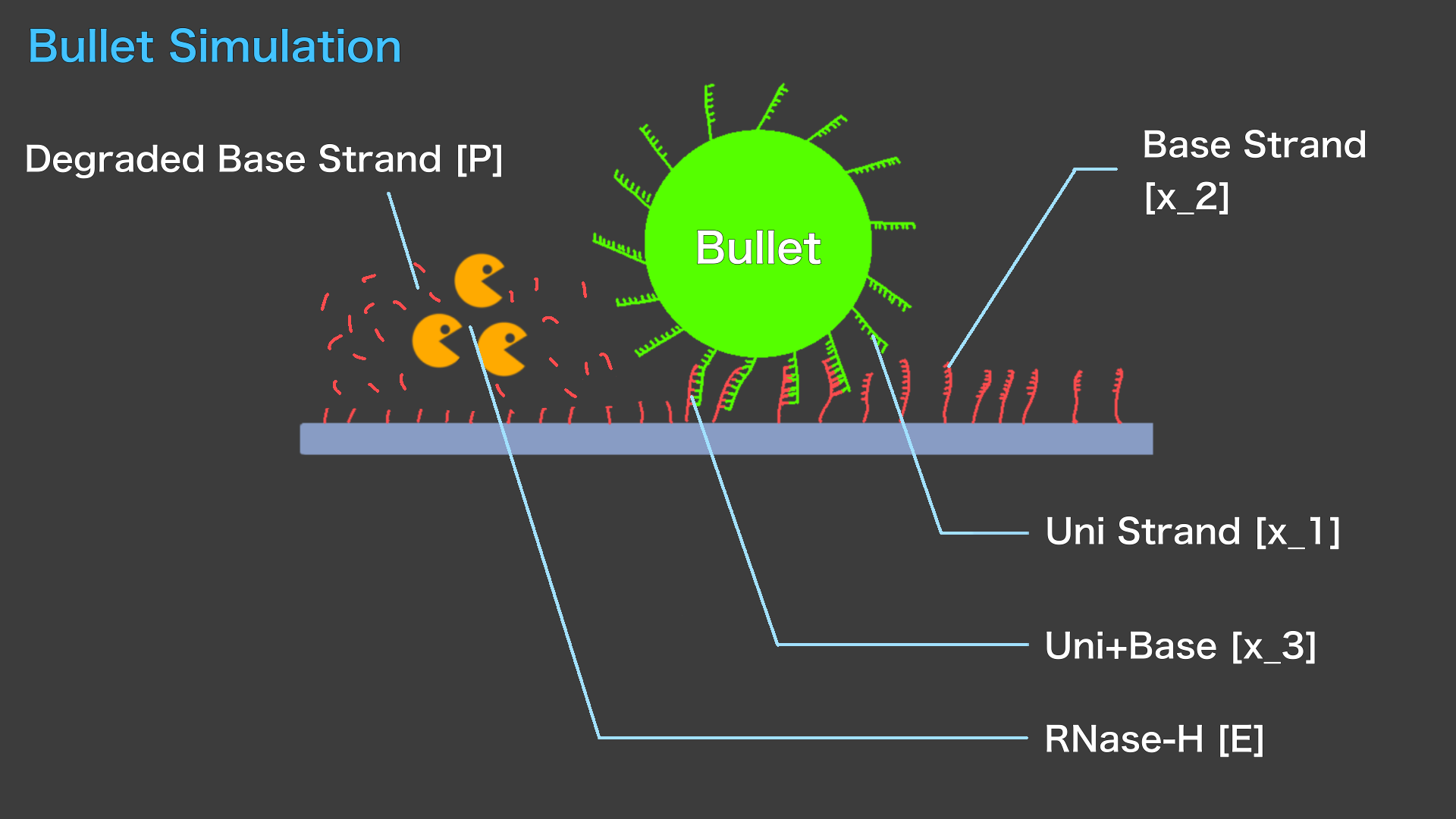
The following model shows how RNase-H actually moves Bullet placed on Field.

\begin{align} X_1 + X_2 &\xrightarrow{k_1} X_3 \\ X_3 + E &\xrightarrow{k_2} P + E \\ \frac{d[X_1]}{dt} &= -k_1[X_1][X_2]+\frac{k_2[E]_0[X_3]}{K_m + [X_3]} \\ \frac{d[X_2]}{dt} &= -k_1[X_1][X_2]+\frac{k_2[E]_0[X_3]}{K_m + [X_3]} \\ \frac{d[X_3]}{dt} &= k_1[X_1][X_2]-\frac{k_2[E]_0[X_3]}{K_m + [X_3]} \\ \frac{d[P]}{dt} &= \frac{k_2[E]_0[X_3]}{K_m + [X_3]} \\ \end{align}

\([X_1]\) : concentration of Uni strand
\([X_2]\) : concentration of Base strand
\([X_3]\) : concentration of Uni/Base double strand
\([E]\) : initial concentration of RNase-H
\([P]\) : concentration of degraded Base strand

The dynamics of Bullet can be inferred from the change in \([X_3]\). \([X_3]\) is extremely low, Bullet will leave the Field and may be sent somewhere far away. If \([X_3]\) is almost equal to the initial \([X_1]\), Bullet may remain stuck in the Field, and the continued presence of a certain percentage of Uni/Base double strand will allow the Bullet to remain on the Field. And when there is a certain amount of Base strand and Uni strand that do not form double strands, Bullet may roll over the Field and move.
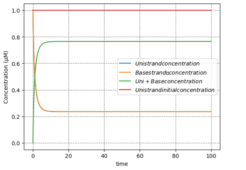
The actual calculations were performed using python. The code used and the results are shown below.

import numpy as np
import matplotlib.pyplot as plt
from scipy.integrate import odeint

#Setting of reaction rate constants

k_1 = 1.0
k_2 = 1.0
k_m = 2.0     # Michaelis constant

#Setting Enzyme Concentration
E = 0.2 


#Differential equations
def nemui1(y,t):
    dydt = [- k_1 * y[0] * y[1] + k_2 * y[2] * E/ (k_m + y[2]),
            
k_1 * y[0] * y[1] + k_2 * y[2] * E/ (k_m + y[2]),+ k_1 * y[0] * y[1] - k_2 * y[2] * E/ (k_m + y[2]),
            0]
    return dydt
x_1 = 1.0  #Uni strand concentration

x_2 = 1.0  #Base strand concentration

x_3 = 0    #Uni+Base concentration

x_4 = 1.0  #Uni strand initial concentration

y = [x_1, x_2, x_3, x_4,]


t = np.linspace(0,100,1000)
y = odeint(nemui1,y,t)


plt.plot(t,y)
plt.xlabel('time')
plt.ylabel('Concentration (µM)')
plt.grid(True, linestyle='--', color='grey')
plt.legend(["$Uni strand concentration$","$Base strand concentration$",
            "$Uni+Base concentration$","$Uni strand initial concentration$"])
plt.rcParams['axes.facecolor'] = 'white'
plt.show()

As can be seen from the above results, when there are extremely large amounts of RNase-H, \([X_3]\) becomes very large and Bullet are fixed on the Field. On the other hand, when RNase-H is extremely low, \([X_3]\) becomes very small and Bullet moves away from the Field. It was shown that by setting the concentration of the RNase-H( \([E]\) ) appropriately, Bullet is able to move in a rotational manner and invade Enemy.

Bullet speed

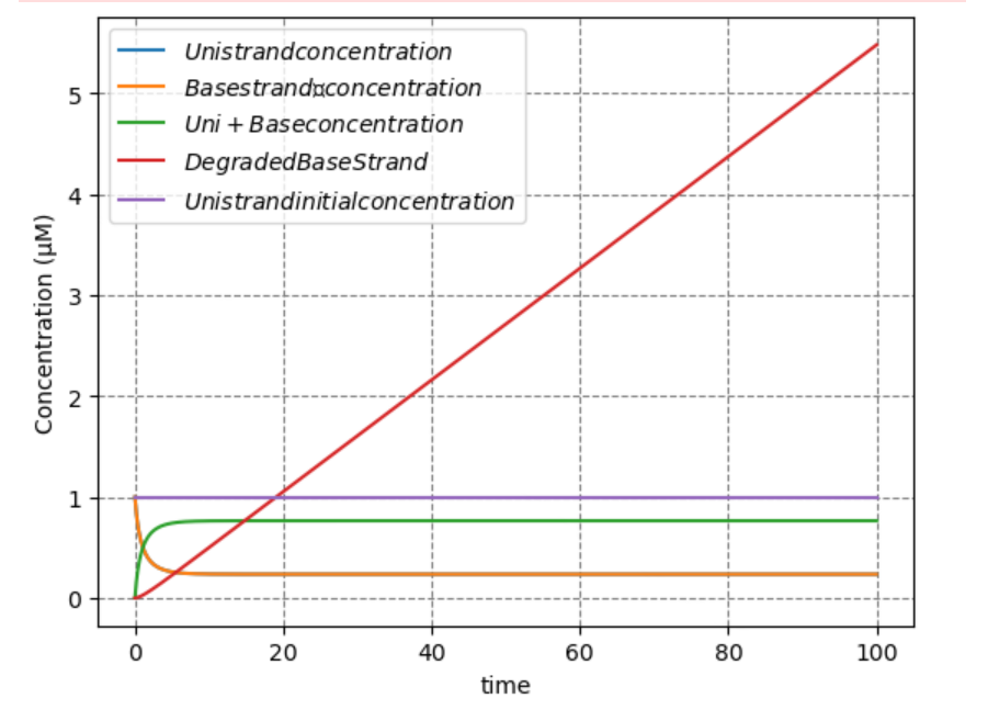
The speed of Bullet can be discussed by considering the change in \([P]\). The code and graph with \([P]\) change are shown below.

import numpy as np
import matplotlib.pyplot as plt
from scipy.integrate import odeint

#Setting of reaction rate constants

k_1 = 1.0
k_2 = 1.0
k_m = 2.0     # Michaelis constant

#Setting Enzyme Concentration
E = 0.2 


#Differential equations
def nemui1(y,t):
    dydt = [- k_1 * y[0] * y[1] + k_2 * y[2] * E/ (k_m + y[2]),
            
k_1 * y[0] * y[1] + k_2 * y[2] * E/ (k_m + y[2]),+ k_1 * y[0] * y[1]
                                        - k_2 * y[2] * E/ (k_m + y[2]),+ k_2 * y[2] * E/ (k_m + y[2]),
            0]
    return dydt
x_1 = 1.0  #Uni strand concentration

x_2 = 1.0  #Base strand concentration

x_3 = 0    #Uni+Base concentration

x_4 = 0    #Degraded Base strand

x_5 = 1.0  #Uni strand initial concentration

y = [x_1, x_2, x_3, x_4,x_5]


t = np.linspace(0,100,1000)
y = odeint(nemui1,y,t)


plt.plot(t,y)
plt.xlabel('time')
plt.ylabel('Concentration (µM)')
plt.grid(True, linestyle='--', color='grey')
plt.legend(["$Uni strand concentration$","$Base strand concentration$",
            "$Uni+Base concentration$","$Uni strand initial concentration$"])
plt.rcParams['axes.facecolor'] = 'white'
plt.show()

The graph of \([P]\) draws a straight line. The slope of the line represents the degradation rate of the Base strand, which is proportional to the speed of Bullet. The equation for \([P]\) indicates that \([P]\) is proportional to \([E]\) and that the speed of Bullet increases as the amount of RNase-H is increased.

Cannon simulation

The sequences of each strands were designed using NUPACK.
The sequences for the Uni strand were taken from Enemy reference paper^[2], since the interaction of the Uni strand with Enemy is also involved.

Sequence Design

DNA / RNA base sequences
Name	DNA/RNA	sequence	bp
Uni	DNA	5'-**AAGAGATTAATTCCG-3'	**+15
Base	RNA	5'-**CGGAAUUAAUCUCUU-3'	**+15
Stopper	RNA	5'-GGGGGAAGAGAUUAAUUCCG-3'	20
Trigger	RNA	5'-CGGAAUUAAUCUCUUCCCCC-3'	20
	is junk sequence,only for extending strand. Each does not represent the same sequence

Base+Uni

Base+Stopper

The Stopper strand and Uni strands hybridize 100% with the Base strand.

Stopper+Trigger

Base

Base+Base

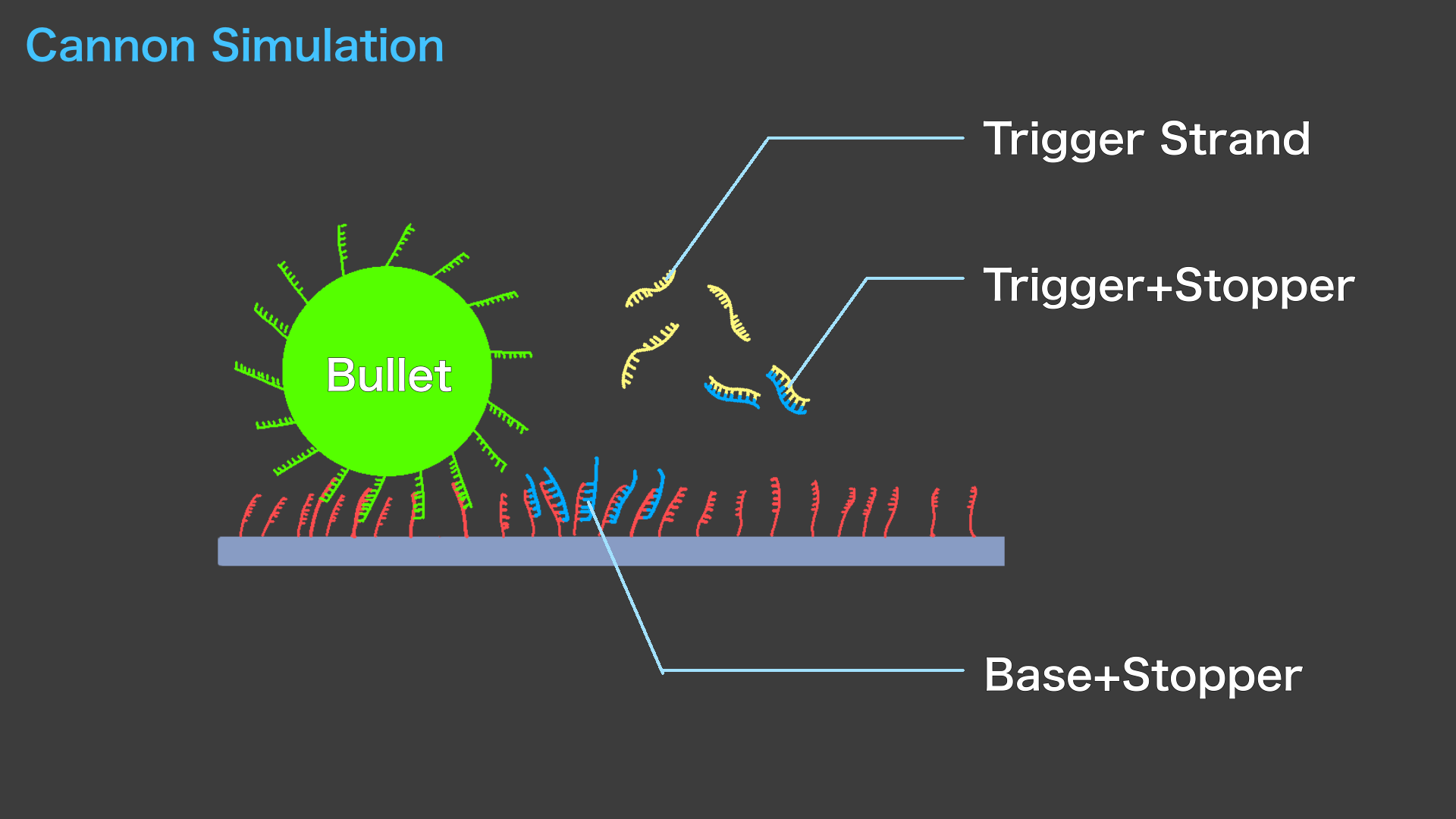
When the Stopper strands, Base strands, and Trigger strands are mixed, the Trigger strand and Stopper strand hybridize 100%. Based on these results, the above sequence was judged to be valid.

Time-Dependent Advancement of Strand displacement

Next, simulations using Visual DSD were performed to verify the strand displacement reaction when a Trigger chain was added. The code and the graphical results are shown below.

directive simulation {initial=0; final=4000; points=1000;plots=[[1]{2^};[1 2^];<1 2^>]}
directive simulator deterministic 
def Trigger() = <1 2^>
def StopperBase() = [1]{2^}
def StopperTrigger() = [1 2^]
def N=10
def N1=1
(N * Trigger()
|N1 * StopperBase()
|0.0 * StopperTrigger())

Result

The reaction is rapid, indicating that the Trigger strand acts as Cannon.